As iron sharpens iron,
so one person sharpens another.
— Proverbs 27:17, New International VersionNote: This post was written with the help of AI.
Four groups of methods
| Direction | Approach | Related work |
|---|---|---|
| Get PPO's batch right | Batch = environment count × steps per environment. Also check whether resets are synchronized, and whether minibatches and learning rates change with environment count. These are the cheapest changes, and the ones most often done wrong. | Rudin · Andrychowicz · DD-PPO · Mayor · Staggered Resets · Hilton · Beukman |
| Multiple policies: diversity through a population | Train several to dozens of policies on one GPU. Let them borrow data, or periodically discard poor ones and mutate good ones. This buys exploration diversity at the cost of more compute and more complex code. | DexPBT · SAPG · EPO |
| Change the starting point: resets and curricula | Put difficult states directly into the batch: start episodes from generated grasp states, intermediate demonstration states or states near the goal, then choose starting points by success rate. This helps most on long-horizon contact tasks. | OmniReset · SGS · DemoStart · RFCL · DextrAH-G/RGB · CSRL |
| Off-policy returns with massive parallelism | Reuse data through replay buffers, with large batches, distributed critics and normalization, making SAC/TD3 faster than PPO with thousands of environments. | PQL · PQN · FastTD3 · FastSAC · FlashSAC/WarpSAC · REPPO |
Timeline of related work
- DD-PPO
- Hilton (PPO-EWMA)
Years follow conference dates, or arXiv dates when there is no conference.
1. On-Policy: getting the batch right
[CoRL'21] Learning to Walk in Minutes Using Massively Parallel Deep Reinforcement Learning
Comment: This is where the well-known rsl_rl / legged_gym comes from.
Paper: arXiv:2109.11978
Code: legged_gym · rsl_rl
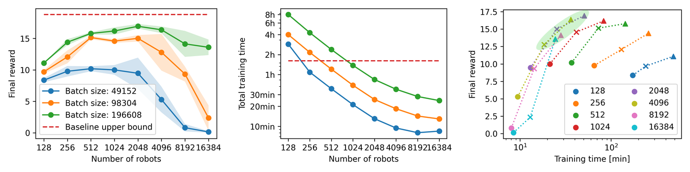
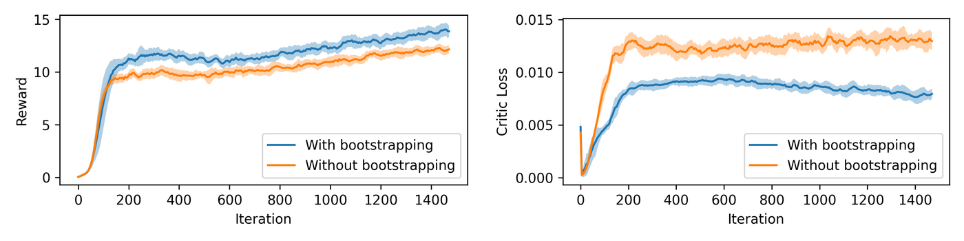
Main takeaway
- Large batch size, large \(N_{\mathrm{env}}\).
- Time-limit truncation should use value bootstrapping.
[ICLR'22] What Matters In On-Policy Reinforcement Learning? A Large-Scale Empirical Study
Paper: arXiv:2006.05990
Main takeaway
A collection of tricks. I don’t see one standout conclusion.
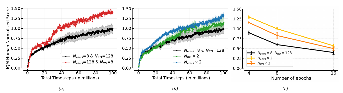
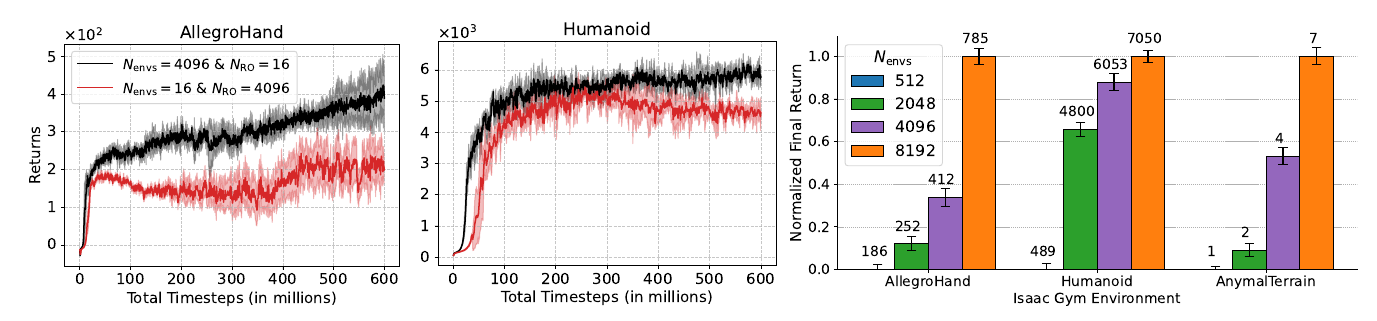
[ICML'25] The Impact of On-Policy Parallelized Data Collection on Deep Reinforcement Learning Networks
Paper: arXiv:2506.03404
Main takeaway
In parallel on-policy RL, batch size is \(|B|=N_{\mathrm{envs}}\times N_{\mathrm{RO}}\). More environments and shorter rollouts work better than the reverse allocation.
[NIPS'25] Staggered Environment Resets Improve Massively Parallel On-Policy Reinforcement Learning
Paper: arXiv:2511.21011
Code: staggered-resets
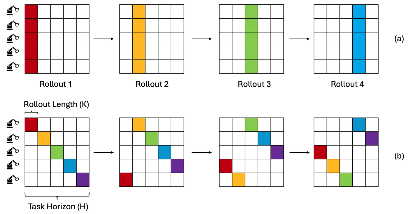
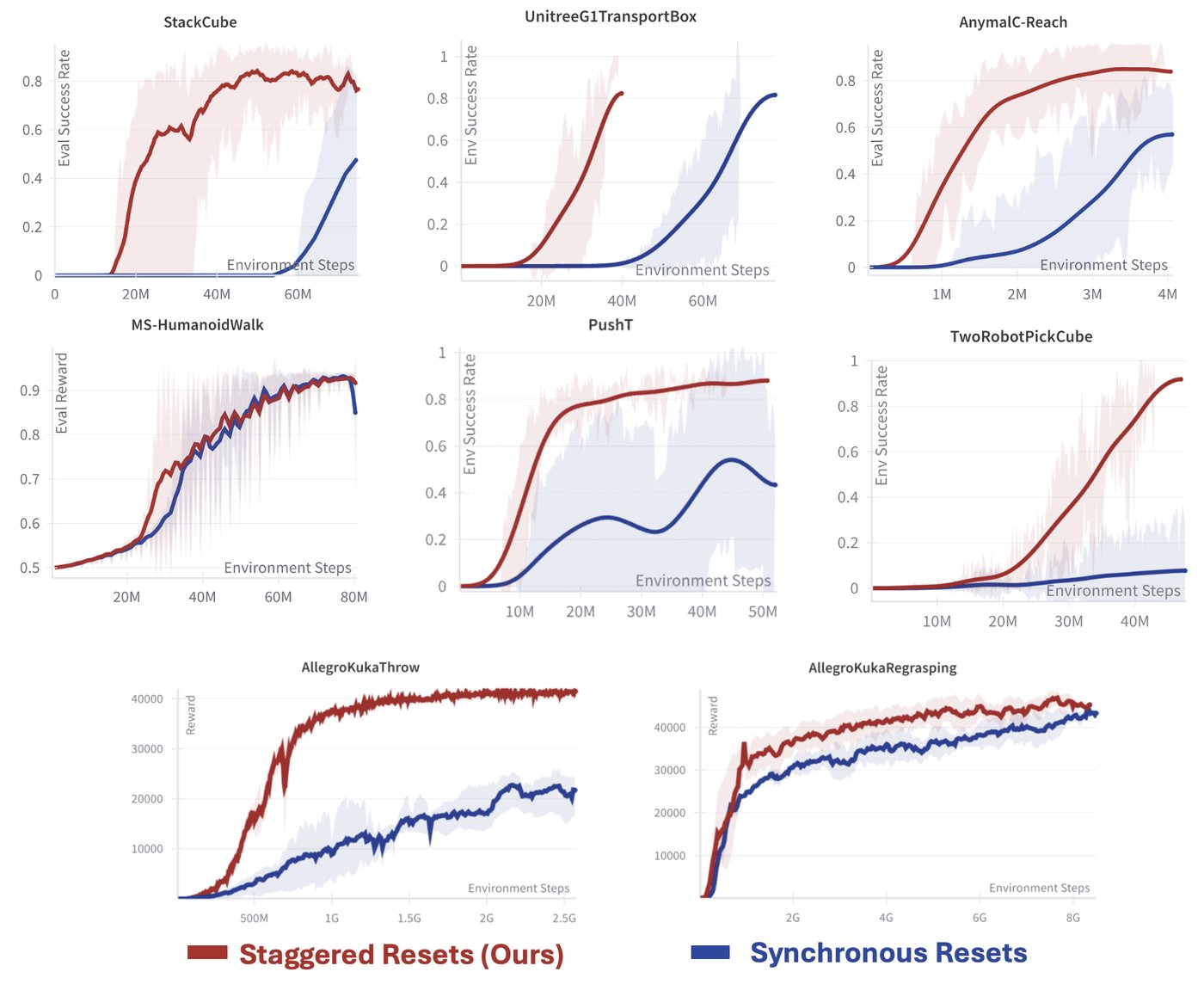
If all environments start together at \(t=0\) and hit the time limit together at \(t=H\), the batch for update \(j\) only contains states in the short window \([(j-1)K,\;jK-1]\). One batch is entirely “just started,” the next is entirely “in the middle of grasping,” and so on. After \(\lceil H/K\rceil\) updates, everything jumps back to the beginning. The authors call this cyclical nonstationarity. The critic keeps chasing a changing distribution, learning later stages and forgetting earlier ones (catastrophic forgetting).
Main takeaway
Stagger the distribution at the initial reset.
2. On-Policy: making use of the fleet
[RSS'23] DexPBT: Scaling up Dexterous Manipulation for Hand-Arm Systems with Population Based Training
Paper: arXiv:2305.12127
Code: Population Based Training in Isaac Lab
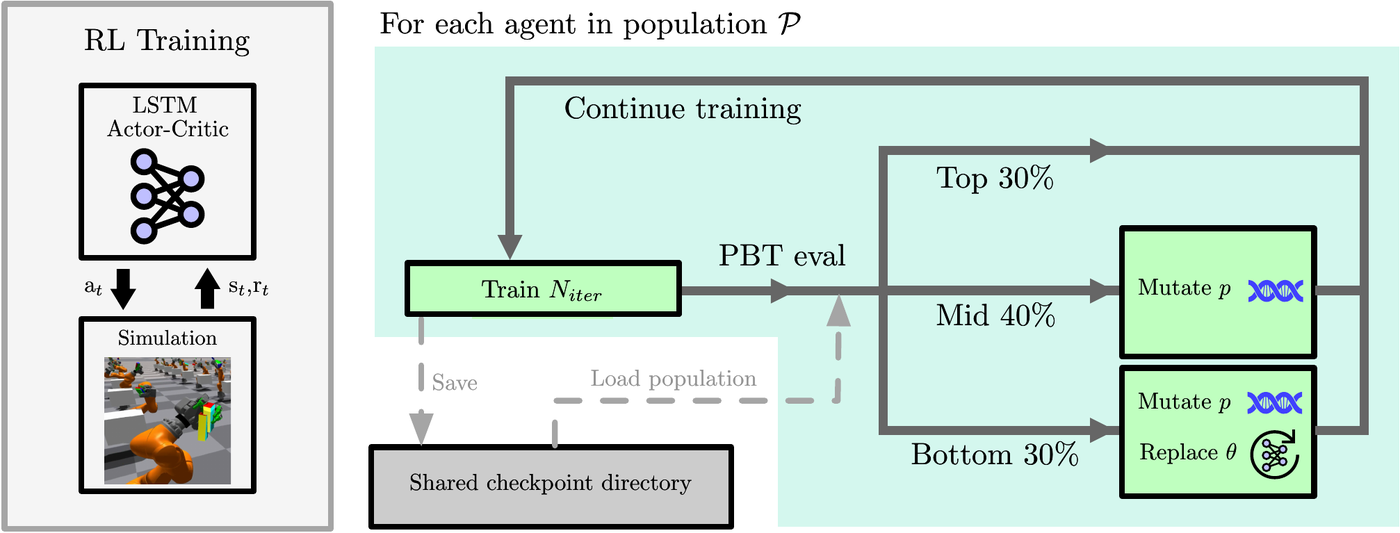
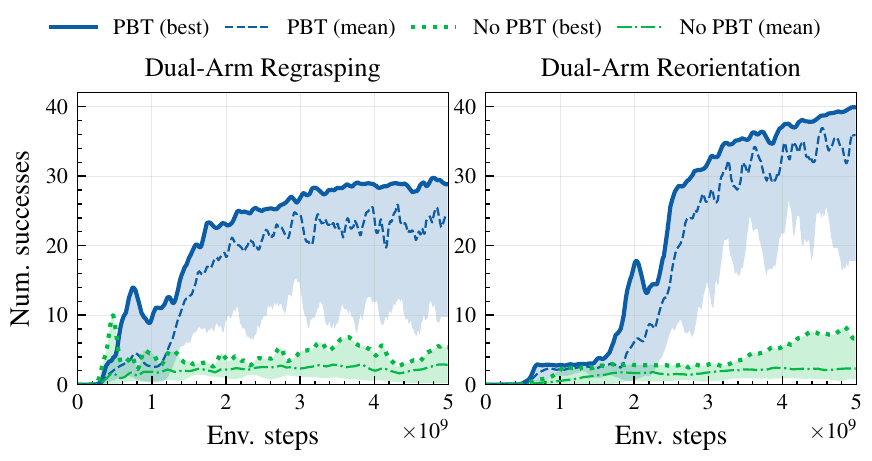
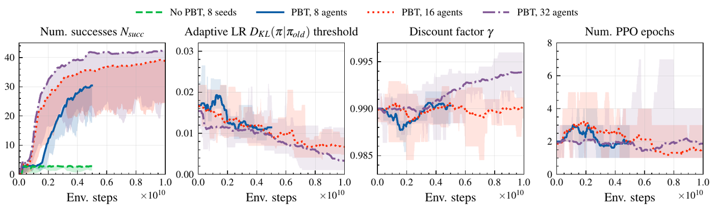
Exploration is difficult in arm-and-multifinger-hand tasks. Run 8–32 PPO trainings at once, each on one GPU with 8,192 environments. Periodically copy good runs into bad ones and randomly perturb hyperparameters and reward coefficients. A population with evolution helps address the local optima that a single PPO run can get stuck in on high-dimensional dexterous manipulation.
Main takeaway
PPO is a lottery, especially on high-dimensional tasks. Buy more tickets, then give the runs that work more room. The outer loop is much like a genetic algorithm.
[ICML'24] SAPG: Split and Aggregate Policy Gradients
Paper: arXiv:2407.20230
Code: sapg
Once PPO’s \(N_{\mathrm{env}}\) gets large enough, increasing batch size further saturates performance (blue: PPO; red: SAPG).
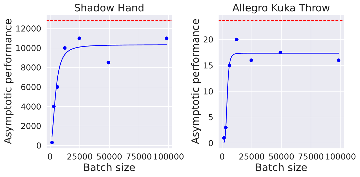
The authors’ explanation is that all environments sample from the same Gaussian policy, so most actions stay near the mean. More environments produce more redundant data: the extra environments are wasted.
Method:
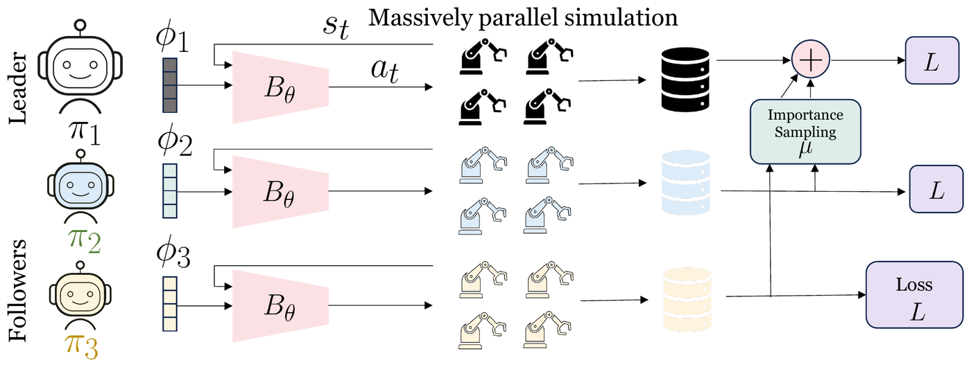
Split: Divide \(N\) environments evenly among \(M\) policies \(\pi_1\ldots\pi_M\). The paper uses \(M=6\) and \(N=24576\), giving each policy 4,096 environments. All policies share actor trunk \(B_\theta\) and critic trunk \(C_\psi\). Policy \(j\) also has its own learnable vector \(\phi_j\), used as an input condition: \(\phi_j\in\mathbb R^{32}\) for complex tasks and \(\mathbb R^{16}\) for simple tasks. Only its own loss updates \(\phi_j\); all losses update \(\theta\) and \(\psi\).
Leader–follower aggregation: \(\pi_1\) is the leader; \(\pi_2\ldots\pi_M\) are followers.
Followers use ordinary PPO on their own block’s on-policy data.
The leader uses an on-policy PPO loss plus \(\lambda\) times an off-policy loss, with \(\lambda=1\). Off-policy data from the followers’ combined data are subsampled to match the amount of the leader’s own data, \(|D'_1|=|D_1|\), so noisier off-policy gradients do not overwhelm the on-policy gradients.
The clipped off-policy surrogate comes from Meng et al. (2023)’s off-policy PPO:
\[ \begin{aligned} L_{\mathrm{off}}(\pi_i;X) &=\frac{1}{|X|}\sum_{j\in X}\mathbb E_{(s,a)\sim\pi_j} \left[\min\left(rA,\;\operatorname{clip}\left(r,\mu(1-\epsilon),\mu(1+\epsilon)\right)A\right)\right],\\ r&=\frac{\pi_i(a\mid s)}{\pi_j(a\mid s)},\qquad \mu=\frac{\pi_{i,\mathrm{old}}(a\mid s)}{\pi_j(a\mid s)}. \end{aligned} \]The clipping interval is shifted around the ratio of the old policy to the behavior policy. \(A\) is the advantage estimated by the leader’s old critic. When \(j=i\), this reduces to ordinary PPO.
The critic uses a 3-step return target for on-policy data and a 1-step target for off-policy data:
\[ \begin{aligned} V^{\mathrm{tgt}}_{\mathrm{on}} &=\sum_{k=t}^{t+2}\gamma^{k-t}r_k+\gamma^3V_{\mathrm{old}}(s_{t+3}),\\ V^{\mathrm{tgt}}_{\mathrm{off}} &=r_t+\gamma V_{\mathrm{old}}(s_{t+1}). \end{aligned} \]Total critic loss = on + \(\lambda\cdot\)off.
Diversity: Besides conditioning on \(\phi_j\), followers can optionally receive different strengths of entropy regularization. Policy \(i\) has entropy coefficient \(\lambda_{\mathrm{ent}}(i-1)\); the leader has none. Each block then has its own learnable \(\sigma\) vector. Choose \(\lambda_{\mathrm{ent}}\) from \(\{0,0.003,0.005\}\): Reorientation and ShadowHand use 0.005; the others use 0.
Each iteration: every block rolls out 16 steps (AllegroKuka), the losses are combined, and \(\theta\), \(\psi\) and \(\phi\) are updated together (Algorithm 1).
Main takeaway
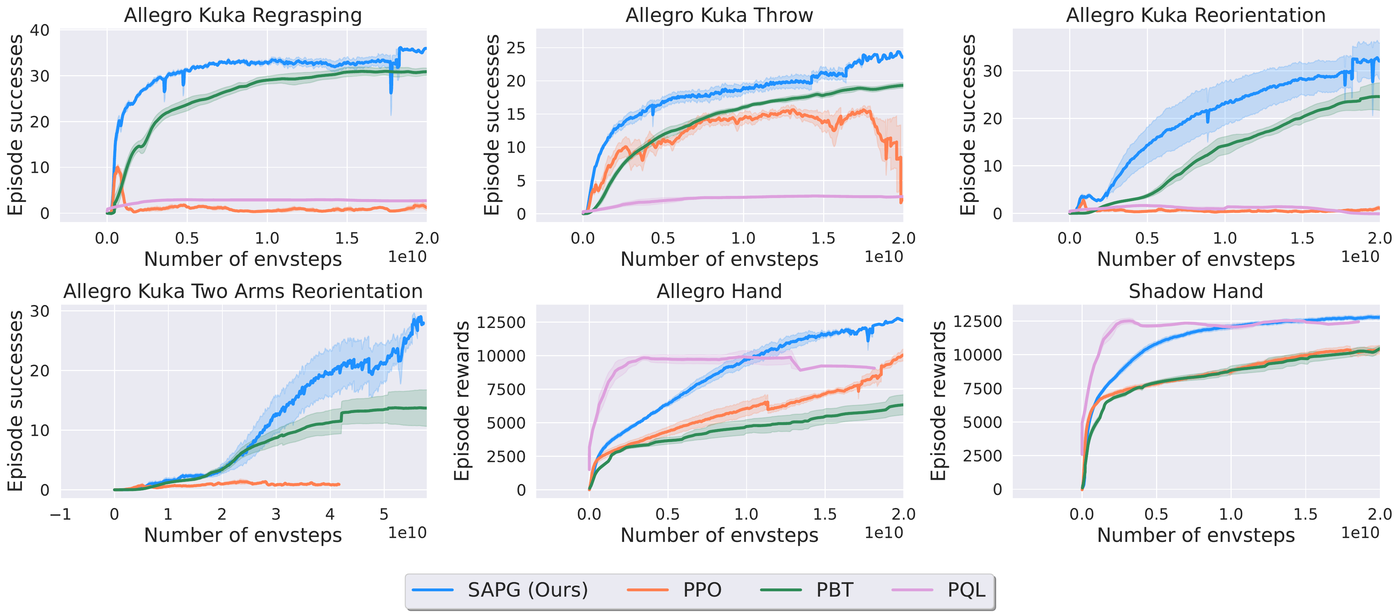
Avoiding redundant sampling in on-policy algorithms improves policy performance.
[arxiv'25] EPO: Evolutionary Policy Optimization
Paper: arXiv:2503.19037
Code: EPO
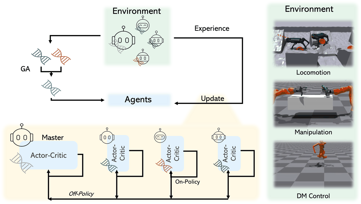
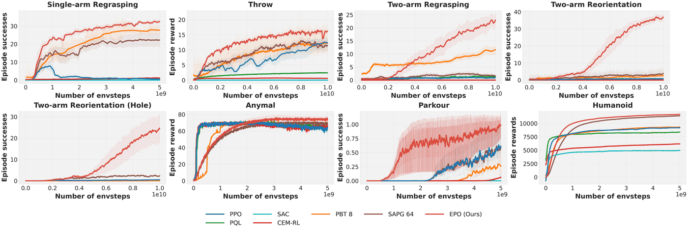
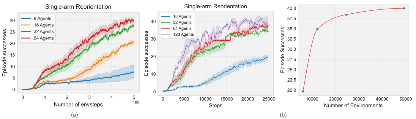
Building on SAPG’s framework where the leader absorbs follower data, EPO increases the number of followers to 64 and applies a genetic algorithm to their latent vectors \(\phi\): discard poor ones, then cross and mutate good ones. This lets the number of policies scale with the environment count.
3. On-Policy: choosing how to reset
[ICLR'26] OmniReset
Paper: arXiv:2603.15789
Code: UWLab
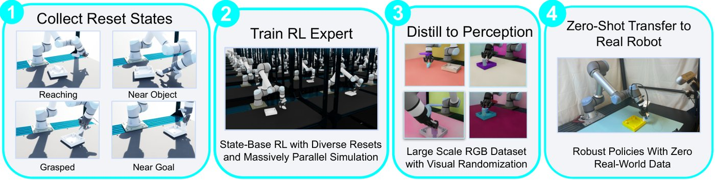
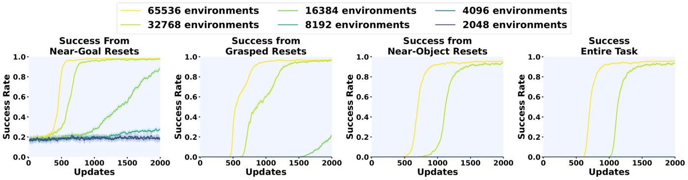
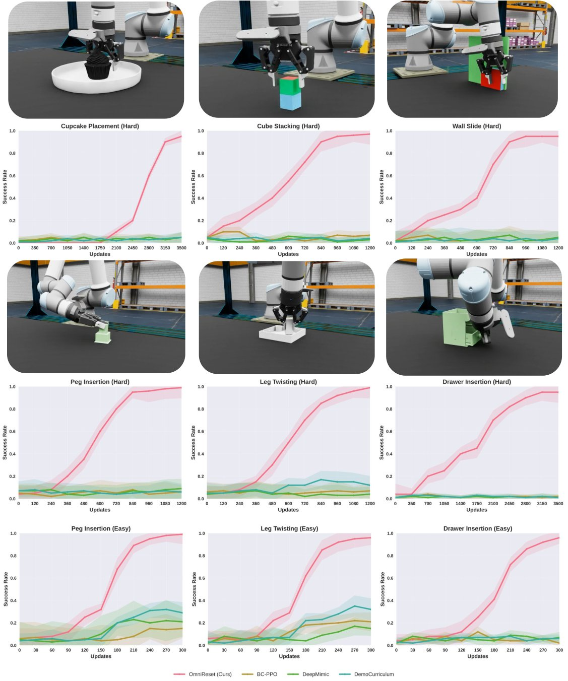
Standard PPO saturates under massive parallelism: more environments keep sampling the same narrow part of the state space. Success signals are too rare in long-horizon tasks, and the policy gets stuck in local optima—for example, only learning to reach.
Method: Procedurally generated diverse reset states + PPO with many parallel environments.
Main takeaway
Large \(N_{\mathrm{env}}\) makes sense. Avoiding redundant sampling makes sense. Manually adjusting the reset distribution to increase coverage and change the transition distribution in the buffer makes sense.
[CoRL'26] SGS-RL
A Balanced Data Diet: Addressing the Exploration Bottleneck in Mega-Scale RL for Robot Control
Paper: arXiv:2610.12465
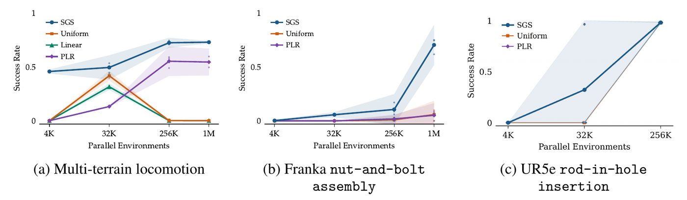
After introducing OmniReset-style diverse resets, uniform sampling spends more and more environments on configurations the policy has already mastered or cannot yet solve. These configurations contribute little to the PPO gradient (advantages are near zero). More environments mean more wasted experience in absolute terms, so the benefit of adding environments disappears or even reverses.
Related: DemoStart: Demonstration-led auto-curriculum applied to sim-to-real with multi-fingered robots filters out demonstration starting states from which previous attempts were all successes or all failures. This is an extreme / degenerate version of the same idea under a different problem setup.
Method:
Before training, sample a fixed set of \(N\) configurations \(\tau_i=(s_0,g,e)\) from the task distribution: initial state, goal and environment. \(N=32768\) for manipulation and \(N=104000\) for locomotion.
For each configuration, keep the outcomes of the last \(H=100\) attempts in a ring buffer. Their mean gives success rate \(p_i\).
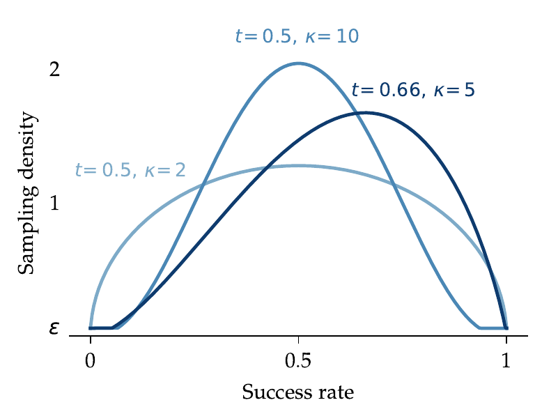
Score configurations with a Beta kernel in mode–concentration form, using target success rate \(t\) and concentration \(\kappa\):
\[ \begin{aligned} w_i&=(p_i+\epsilon)^{\kappa t}(1-p_i+\epsilon)^{\kappa(1-t)},\\ \ell_i&=\log(\max(w_i,\epsilon)+\epsilon). \end{aligned} \]At the end of each episode, sample the next configuration with a softmax. The implementation uses \(T_{\mathrm{eff}}=\max(T,1)\):
\[ p(i)=\frac{\exp(\ell_i/T)}{\sum_j\exp(\ell_j/T)},\qquad T_{\mathrm{eff}}=\max(T,1)\quad\text{(implementation)}. \]Hyperparameters: \(H=100\), \(T=2\). Manipulation uses \(t=0.5\), \(\kappa=1\), \(\epsilon=10^{-4}\); locomotion uses \(t=0.66\), \(\kappa=5\), \(\epsilon=10^{-8}\). \(\epsilon\) ensures every configuration has nonzero probability, allowing its success-rate estimate to keep being updated.
Other choices: one shared reward within each domain, consisting of terminal success plus small regularization terms. The number of PPO minibatches stays fixed, so batch size grows proportionally with environment count.
For manipulation, the reset pool uses OmniReset’s three categories: Reaching, Stable Grasp and Near-Goal, each making up one third. Collision checks are done in advance.
Relation to existing methods: the idea is shared with Sampling for Learnability (SFL), which scores with \(p(1-p)\). The differences are a sliding-window success rate, an adjustable target success rate and a minimum probability for every configuration. PLR, another comparison, scores with \(|\mathrm{GAE}|\).
Main takeaway
States that are too hard or too easy have little learning signal. This is adaptive sampling that resets into states of moderate difficulty.
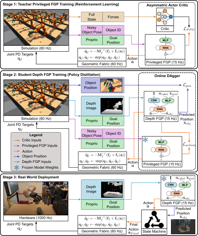
[CoRL'24] DextrAH-G / DextrAH-RGB
DextrAH-G: Pixels-to-Action Dexterous Arm-Hand Grasping with Geometric Fabrics
- Paper: arXiv:2407.02274
DextrAH-RGB: Visuomotor Policies to Grasp Anything with Dexterous Hands
- Paper: arXiv:2412.01791
- Code: DEXTRAH (“DextrAH on Isaac Lab,” including privileged RL and online distillation)
Direct joint-space PPO for high-dimensional arm-and-multifinger-hand actions trains slowly, learns unnatural grasps (such as holding an object between the middle and ring fingers), fails to learn with multiple objects and is unsafe on hardware.
Method: Replace 23-dimensional joint actions with 11-dimensional palm-pose + hand-PCA-synergy actions, while handling collision avoidance and joint limits.
Main takeaway
Reducing a high-dimensional action space can substantially improve learning speed. Dexterous Functional Grasping (EigenGrasp) uses a similar idea.
Follow-up: EigenDEXplore uses eigenvectors to aid exploration, with somewhat softer constraints.
4. Off-Policy notes
Mega-Scale RL is still mostly on-policy. Off-policy has attracted renewed interest recently, especially after FlashSAC. Here are representative works and their main insights.
[ICML'23] PQL — Parallel Q-Learning: Scaling Off-policy Reinforcement Learning under Massively Parallel Simulation
Split DDPG into three parallel processes: an actor collects data, a V-learner learns Q and a P-learner learns the policy. This lets off-policy RL use tens of thousands of Isaac Gym environments on one workstation, with shorter wall-clock time and better sample efficiency than PPO.
Paper: arXiv:2307.12983
Code: pql
Main takeaway
Different exploration strengths for different environments are worth trying.
[ICLR'25] PQN: Simplifying Deep Temporal Difference Learning
Paper: arXiv:2407.04811
Code: purejaxql
Shows that LayerNorm, plus a small amount of \(\ell_2\) regularization, lets TD learning converge without a target network or replay buffer. DQN becomes pure GPU Q-learning with many parallel environments, short \(\lambda\)-returns and PPO-like minibatch updates.
Main takeaway
LayerNorm and \(\lambda\)-returns both matter.
[arxiv'25] FastTD3: Simple, Fast, and Capable Reinforcement Learning for Humanoid Control
Paper: arXiv:2505.22642
Code: FastTD3
No new invention: turn PQL’s lessons into a synchronous, simple, well-tuned TD3. Parallel simulation + huge batches (32,768) + categorical critic + CDQ solves most HumanoidBench tasks within three hours on one A100, with support for IsaacLab / MuJoCo Playground.
Main takeaway
Large batches and a categorical critic make sense.
[arxiv'25] FastSAC: Learning Sim-to-Real Humanoid Locomotion in 15 Minutes
Paper: arXiv:2512.01996
Code: holosoma
Stabilizes the FastSAC variant that was unstable in the FastTD3 paper. With a minimal reward, one RTX 4090 trains a G1/T1 whole-body walking policy (29 degrees of freedom) in 15 minutes, with strong domain randomization and hardware transfer. Whole-body motion tracking with 4×L40S and 16,384 environments is also faster than PPO.
Main takeaway
LayerNorm, Q-mean rather than CDQ, and automatic alpha.
[RSS'26] FlashSAC: Fast and Stable Off-Policy Reinforcement Learning for High-Dimensional Robot Control
- Paper: arXiv:2604.04539
- Code: FlashSAC
Main takeaway
Use a larger network (2.5M parameters, six layers), larger batches and a larger replay buffer, with fewer gradient updates (UTD = 2/1024). Then constrain norms with BatchNorm, RMSNorm, weight projection and a distributional critic, making SAC fast and stable on high-dimensional tasks.
Follow-up: WarpSAC: Towards the Pinnacle of Scalable Off-policy RL by Rethinking Exploration and Exploitation
- Paper: arXiv:2608.24479
- Code: warprl
Main takeaway
Under massive GPU parallelism, turning off weight-projection normalization and using a single Q works better.